Executive Summary: Granularity and precision in VM-22 asset modeling
VM-22 increases the modeling burden for annuity insurers by requiring stochastic asset and liability projections for asset-intensive business. For many insurers, the key challenge is not simply building a compliant model but doing so in a way that captures the asset-liability management (ALM) interactions that drive reserve results without creating impractical runtimes.
This paper outlines an asset modeling playbook that distinguishes between characteristics that require seriatim treatment and those that can be aggregated, externally projected, or clustered. The framework focuses on two decision points: maintaining enough granularity to support disinvestment, collateral, and default assumptions, and maintaining enough precision to capture path dependency, optionality, and structured-asset cash flows.
The illustrative case study shows that clustering can reduce runtime while preserving valuation accuracy. A portfolio including callable and non-callable bonds was compressed 10-to-1 and achieved a close fit on cash flow along with a VM-22 reserve within 0.136% of the seriatim result. The practical takeaway is clear: With appropriate fit testing and governance, asset compression can free capacity for sensitivity analysis, forecasting, stress testing, and strategic asset allocation without abandoning actuarial rigor.
Introduction: How can insurers increase efficiency for asset-intensive modeling under VM-22?
VM-22 is reshaping how annuity insurers approach pricing, valuation, risk management, and asset-liability analysis. Although stochastic modeling is familiar to insurers with life or variable annuity business subject to principle-based reserving (PBR), many asset-intensive annuity blocks now entering VM-22 require greater stochastic asset modeling capability than legacy processes were designed to support.
That challenge is arriving as insurers hold broader and more complex asset portfolios. Structured assets, private credit, whole loans, and other assets with path-dependent cash flows can improve portfolio economics, but they also increase modeling complexity. Under VM-22, the asset model must support stochastic valuation while preserving the cash flow behavior, market value dynamics, default assumptions, and ALM interactions that drive reserve results.
Efficient asset modeling therefore becomes more than a runtime exercise. Insurers should ensure that their VM-22 models are well-equipped not just for periodic baseline valuation needs, but also for sensitivity analysis, business forecasting, stress testing, and possibly hedging grids. Further, within the VM-22 calculation or other applications of stochastic analysis, insurers may need projected key rate duration or other Greeks that require nested calculation, such as simulation of a dynamic hedge program or reinvestment strategies. The techniques available to reduce runtime can be valuable for these analyses, but only when they are calibrated to ALM-relevant metrics and validated against the reserve outcomes they are intended to approximate.
This paper discusses a practical framework for deciding where asset detail matters most and how granularity and precision should be evaluated, and illustrates how clustering can be applied to reduce asset portfolio size without materially distorting VM-22 results. It also highlights governance considerations and limitations that actuaries should address before relying on compression techniques in production valuation or strategic analysis.
Playbook Step 1: Categorizing the asset portfolio
Insurers’ portfolios increasingly include allocations to structured assets, whole mortgage loans, various forms of private credit, and other Schedule BA investments.1 These assets can improve portfolio economics, but they also increase the variety and complexity of positions to model under VM-22. One notable example is the increased volume of residential mortgage loans (RMLs) on insurers’ balance sheets. Because these assets typically have smaller notional amounts, insurers must hold more individual positions to achieve the same level of investment, increasing the volume of assets that must be modeled. For precise seriatim asset modeling, this creates inefficiencies in modeling.
The intricacies of each asset class can be categorized into several key characteristics that influence the makeup of assets’ modeled cash flow patterns, as summarized in Figure 1.
Figure 1: Key asset characteristics in VM-22 modeling
| Asset characteristic | Consideration |
|---|---|
| Fixed versus floating coupon | Assets with floating coupons will naturally have path-dependent investment income, whereas fixed coupon bonds may be represented by static cash flow streams. |
| Structured versus individual loans | Structured products derive their cash flows from an underlying collateral pool and the security’s contractual waterfall, requiring assumptions about collateral performance, tranche structure, and payment priority. These assets are therefore often modeled using specialized third-party platforms such as Moody’s or Intex. Direct whole loans, by contrast, can generally be modeled individually using loan-level terms and borrower or collateral attributes maintained in the insurer’s investment records. |
| Public versus private credit | Public assets have well-documented terms and conditions to support proper modeling, whereas private deals may have limited documentation or require bespoke modeling. |
| With versus without optionality | Optionality, including both prepayment and extension risk as well as callability, introduces path dependency in the cash flows and necessitates monitoring of asset convexity in ALM practices. |
These contrasting characteristics can be prioritized in insurers’ VM-22 stochastic asset models through the lens of granularity and precision. Seriatim modeling provides the highest level of asset detail, but insurers can often reduce runtime by preserving granularity and precision only where they materially affect ALM behavior and reserve outcomes.
Step 2: Defining VM-22 Asset Portfolio Granularity
Aggregating assets without path dependency, such as “vanilla” government bonds and many corporate bonds, into externally projected asset (EPA) datasets is a relatively straightforward approach to reducing asset portfolio granularity to free up runtime. Alternatively, as discussed later in this paper, compression techniques that reduce the seriatim data into a smaller number of model cells could also be considered. While EPAs have the advantage of maintaining full accuracy of the underlying group of assets, compression methods sacrifice CUSIP-level accuracy for a more optimal runtime across the portfolio.
The modeled granularity of the asset portfolio is important for the application of assumptions and logic critical to the ALM framework within VM-22 PBR such as the disinvestment strategy, defaults, and explicit hedging. When asset cash flows do not sufficiently match projected liability needs, VM-22 models may need to sell existing assets. Many insurers optimize the asset sales process by assigning sale priority to groups of assets, as opposed to pro-rata selling the portfolio. Use of compression or EPAs should incorporate sale priority of assets within any aggregation to prevent modeling of a suboptimal or unrealistic disinvestment strategy. Additionally, when assets are sold and the proceeds are recognized based on market value, an EPA process that collapses cash flows prior to performing granular market value calculations could materially affect the accuracy of the modelling of disinvestment. Similarly, credit quality matters. The model should retain sufficient credit quality information to apply VM-22 default assumptions appropriately across the portfolio. Any aggregation or compression methodology should be cautious grouping assets in a manner that obscures material differences in credit risk or results in the inappropriate application of default assumptions. If a hedge strategy is modeled, sufficient asset-level granularity is necessary to reflect its collateral requirements, including which assets are eligible to be posted, apply the appropriate asset-specific haircuts, and capture the resulting liquidity needs and the knock-on effect to the reinvestment and disinvestment modeling. The intersection of these requirements limits the level of asset aggregation that can be achieved without potentially oversimplifying the model’s ALM mechanics.
Emphasizing portfolio granularity also ensures realistic distribution of asset cash flows. This is particularly relevant in strategic asset allocation (SAA) analysis where insurers or asset managers are evaluating candidate portfolio mixes to optimize yield subject to a few constraints. In this context, it is not uncommon to use a few representative asset cells centered around benchmark yields and maturities. However, this can create unrealistic ALM outcomes when evaluated alongside smooth liability cash flow patterns. In contrast, generating candidate portfolios with a large number of model cells and incorporating ALM metrics into a fitting process for aggregation or compression can lead to more realistic VM-22 reserve measurements.
Step 3: Evaluating the trade-off for precision with complex assets
For assets with path dependency, bespoke terms and conditions, or other complex factors, the precision of the asset cash flows should be weighed against possible simplifications. Compression techniques like clustering should evaluate fit based on robust ALM metrics, including key rate duration and convexity, as opposed to more rudimentary categorical variables. For example, aggregating a sleeve of RMLs could prove problematic due to the idiosyncratic prepayment risks of the asset class, where prepayment rates at a weighted-average coupon for a representative RML could lead to a different cash flow pattern compared to the sum of cash flows from individually modeled loans.
Going further, structured assets or private credit might be simplified through native modeling with more vanilla structures tied to a coupon rate and maturity date based on the asset’s weighted average life (WAL), as opposed to incorporating first-principles cash flow modeling from Moody’s, Intex, or similar platforms. This “bullet bond” approach misses the optionality and detailed cash flow patterns underlying the actual investment but could be sufficiently aligned with expected cash flow patterns. However, when greater precision is needed and additional data is available, modelers can use more sophisticated approaches for structured assets. To better align with structured asset cash flows for compressed cells or private deals, a nearest-neighbor mapping approach could be utilized, where each modeled cell representing structured assets could be mapped to a public structured asset using statistical methods based on the characteristics of the modeled cell.2
VM-22 provides specific guidance on how insurers should demonstrate reasonability in modeling simplifications or approximations, reinforcing the importance of balancing modeling granularity and precision against potential runtime savings.3 Insurance stakeholders, especially appointed actuaries (or the qualified PBR actuaries) signing off on actuarial memoranda, should also be wary of employing techniques that fail to capture the risks associated with the growing complexity in asset portfolios and ensure that their models are sufficiently rigorous to meet the requirements of actuarial standards of practice (ASOPs). With thoughtful methodologies, validation, and governance, utilizing modeling efficiency techniques like clustering can unlock analytical capabilities that deliver strategic insights for VM-22 beyond point-in-time valuation.
Case study: Asset portfolio clustering in VM-22
To illustrate one approach for effectively reducing the size of the asset portfolio, we explore the application of the clustering technique designed to meet key risk metrics while still reducing the runtime strain. The clustered asset portfolio preserves sufficient granularity across asset types, enabling the insurer to evaluate SAA alternatives efficiently while maintaining cash flow precision. This case study examines a portfolio of fixed-coupon bonds, many of which have a callable provision that introduces some optionality in the cash flows, as shown in Figure 2. This portfolio is assumed to be supporting a payout annuity block with fixed liability cash flows, utilizing principle-based VM-22 reserving.
Figure 2: Asset portfolio summary
| Bond type | Cells | Par value ($ million) | Par % |
|---|---|---|---|
| Non-callable | 695 | $2,343 | 40.6% |
| Callable at par | 832 | $2,806 | 48.6% |
| Callable with premium | 80 | $626 | 10.8% |
| Total | 1,607 | $5,775 | 100.0% |
Clustering is a compression technique that reduces a large set of data into a group of data points algorithmically based on the similarity of features between the data. When applied to the seriatim asset portfolio, similar assets are identified using a set of location variables and are grouped together, with one cell selected to represent each group. The representative cells are then scaled up so that aggregate portfolio totals are preserved. With this model, the seriatim asset portfolio was compressed by a 10:1 ratio to only 161 modeled cells.
This clustering model uses 15 total location variables, with weights assigned to prioritize fit for variables expected to drive the VM-22 results most significantly. Figure 3 summarizes these location variables, the relative weight assigned, and the goodness-of-fit percentage, showing how close the clustered data aligns with the seriatim. The weightings assigned were judgment-based but alternatively could be determined using an empirical method. It is also worth noting that this model does not assume any differences in sale priority across the portfolio, which would require clear segmentation constraints. In contrast, default assumptions on the other hand, are assumed to be reasonably appropriate based on the spread/credit related location variables included in the clustering model.
Figure 3: Location variables, weights, and fit results from the clustering run
| Category | Variable | Weight | Fit % |
|---|---|---|---|
| Size & value | Par value (time 0) | 20 | 100.0% |
| Book value (time 0) | 10 | 100.0% | |
| Book value (year 10) | 6 | 99.8% | |
| Book value (year 20) | 4 | 100.0% | |
| Book value (year 30) | 2 | 96.9% | |
| Cash flow profile | Cumulative PV of asset CF | 20 | 100.0% |
| Cumulative PV coupon income | 10 | 99.9% | |
| Cumulative PV scheduled principal | 10 | 99.9% | |
| Key rate duration (KRD) | KRD 5-year bucket | 4 | 93.4% |
| KRD 10-year bucket | 6 | 95.5% | |
| KRD 20-year bucket | 4 | 96.3% | |
| KRD 30-year bucket | 2 | 95.2% | |
| Spread/credit | PBR spread input | 10 | 94.9% |
| Option-adjusted spread | 8 | 96.2% | |
| Optionality | Years to call (YTC) | 15 | 97.7% |
Figure 4 illustrates the resulting cluster representatives mapped across two of the location variables—YTC and the cumulative present value of total asset cash flows—where each larger marker denotes a representative cell standing in for a group of similar seriatim assets. Premium-callable bonds form a distinct cluster near YTC = 0, reflecting their imminent call dates and high homogeneity, and were effectively consolidated from 20 unique bond definitions into a single representative cell, reflecting the algorithm's consolidation of bonds that are tightly clustered in location-variable space. Par-callable and non-callable bonds share a similar distribution along the YTC axis in this portfolio, as many par-callable bonds carry call dates close to maturity, and are distinguished in the chart by color. Their separation in location-variable space is driven primarily by cash flow profile and rate sensitivity rather than YTC alone.
Figure 4: Visualization of cluster representatives across the asset portfolio
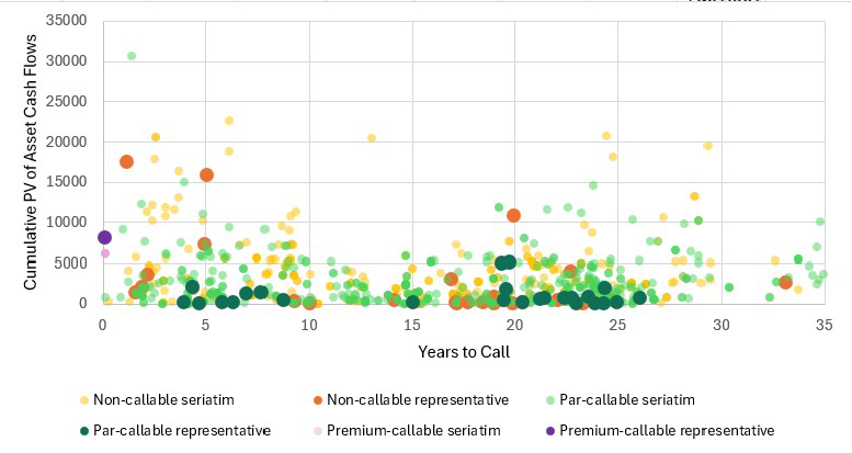
The clustered portfolio resulted in a fit above 99% for the present value of asset cash flows along the median VM-22 scenario, and only a 0.136% difference from the VM-22 reserve using the seriatim asset portfolio, representing a strong alignment. Deeper investigation into the tail scenarios revealed the deviation was driven by a few scenarios with extreme rate volatility that likely triggered the call provisions on a significant portion of the portfolio, leading to differences in timing of reinvestment and reinforcing the importance of incorporating asset optionality measures into clustering criteria. Further refinements could be explored to better calibrate the clustered portfolio for the VM-22 stochastic reserve measure, including greater emphasis on asset optionality or more targeted fit on the subset of stochastic scenarios driving the reserve requirement.
Conclusion
As insurers’ asset portfolios grow more complex and heterogeneous, VM-22 requires a deliberate playbook for deciding where seriatim asset modeling is necessary, where aggregation or clustering is appropriate, and how each simplification should be validated against ALM behavior and reserve outcomes. With a governed approach to portfolio construction, fit testing, and model refinement, insurers can manage stochastic modeling constraints while preserving decision-useful accuracy and gaining deeper insight into the ALM implications of their balance sheets under VM-22.
1 More detailed trends in insurers’ asset holdings were compiled and represented in this publication: Asset allocations and investment strategies of U.S. life insurers in an inflationary interest rate environment.
2 For more details, this whitepaper is a strong reference: Bridging the private-credit modeling gap: A nearest-neighbor approach for insurers.
3 See Valuation Manual, VM-22 Section 3.J. Guidance Note.